You can capture tons of data. Now what?
Offering huge new capabilities is not always seen positively. Sometimes, engineers come to us and ask:
‘Now that I am able to collect Gigabytes of trace data from FPGA running at speed… how do I analyze that much data?’.
Does EXOSTIV just displace the problem?
No, it does not.
In this post, I’ll show:
1) why it is important to enlarge the observation window. – and:
2) how to make the most of this unprecedented capability, based on EXOSTIV Dashboard’s capture modes, triggers and data qualification capabilities.
Random bugs happen
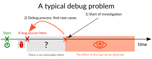
The figure below shows a typical debug scenario. A bug occurs randomly ‘some time’ after system power up. During an initial time interval, the effects of the bug are not noticeable – after which, the system’s behaviour is sufficiently degraded to obviously see the bug’s effect. Typically, the engineer will need to detect a ‘start of investigation’ condition from which he’ll have to ‘roll back in time’ – ultimately to find the root cause of the bug. In the case of an FPGA the engineer observes the FPGA’s internal logic.
Random bugs typically occur as a result of a simulation model issue. The system’s environment could not be simulated with complete accuracy and/or some part of the system behaves differently than initially thought int he ‘real world’. In addition, long operating times are not really the ‘simulation’s best friend’.
Size matters.
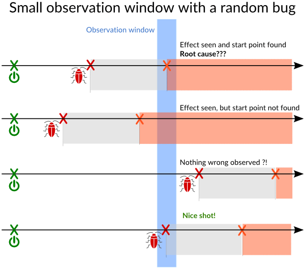
Suppose that we capture some ‘observation window’ of the system. If we are lucky enough to observe a bug right when it occurs, we can get an understanding of what happens. Similarly, we are able to recognize the effects of the bug, as shown by the orange ‘X’ on the picture (called ‘start of investigation). Conversely, we have no idea about how to trigger on such conditions (if we had the ability to trigger on unknown and random bugs, they would have been corrected already).
With a reduced observation window, the process of debugging requires some luck. We can miss everything, recognize an effect without having sufficient data to find the start of investigation. We can be lucky enough to find the start of investigation but no history to roll back to the root cause… – Or: we can hope to ‘shoot right on the bug’.
You do not want to leave the debugging process to chance?
Enlarge the observation window!
VS.
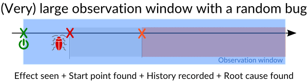
With a properly sized observation window, you can be certain of finding a random bug.
Not ‘brute force’ only
EXOSTIV provides a total observation window of 8 Gigabytes.
However, EXOSTIV is not a ‘brute force’ solution only. Many of its features are equally important to implement ‘smarter’ captures in the lab.
Trigger, Data Qualification, Streaming and Burst help you define better capture windows.
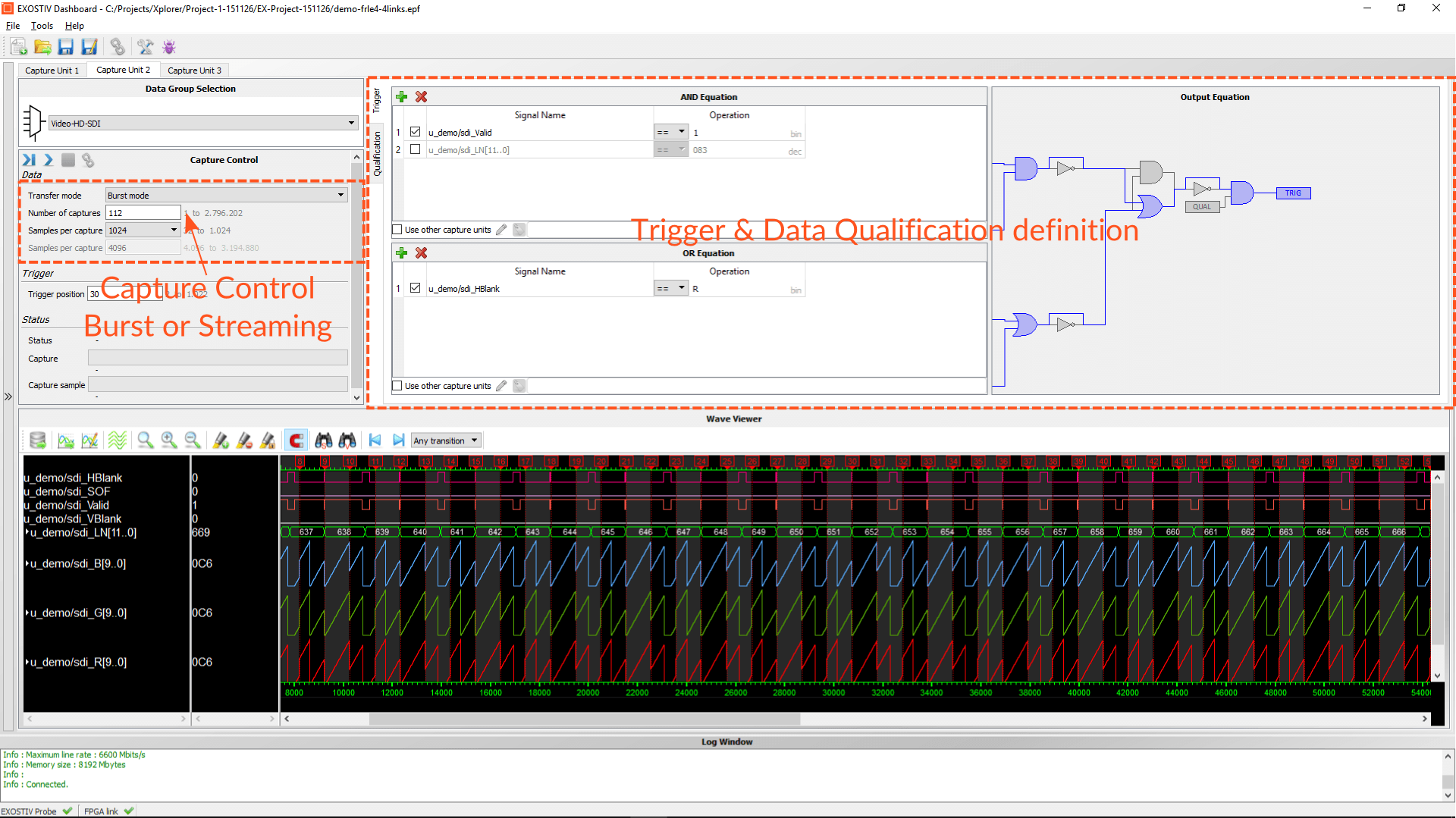
1. Trigger
The total capture window may be gigantic, a triggering capability remains essential. During EXOSTIV IP setup, the nodes that need to be observed are optionally marked as ‘source for trigger’. Currently, EXOSTIV is able to implement a single or repeating trigger based on AND and OR equations defined on these signals. The AND and OR equations can also be combined.
With the growing complexity of systems, defining a very accurate trigger condition has sometimes become a way to overcome a too limited capture window.
This time is over. You are now able to use trigger to collect a better capture window. Maybe you can relax a little bit about defining complex triggering, because you can count on a very large capture window to collect the information that you need.
A unique and extremely useful capability of Exostiv is the ability to define cross-clock domain triggers. In other words, you can detect an event in one clock domain and forward to another clock domain for further capture and analysis. This is the topic of another article (click here if you are interested).
Finally, if you are interested in one among many trigger events, you can think about trigger counters too! At core insertion, you can define some additional resources and add a trigger counter to a capture unit trigger machine. When capturing, you can then carefully select which trigger event you are interested in.
2. Data Qualification
‘Data qualification’ enables you to define a logic condition on the observed signals. Data is captured and recorded by EXOSTIV only when this condition is true.
For instance, this can be used to filter out the times when nothing happens on a bus. This is a very powerful feature that helps you preserve the bandwidth that you use to extract data.
3. Streaming or Burst?
EXOSTIV provides 2 modes of capture:
- Streaming mode: data is captured continuously. If the bandwidth required to capture data exceeds its EXOSTIV Probe capabilities, it stops and resumes capture once it is able to do so. Triggers and capture length can be used to define a repeating start condition.
- Burst mode: data is captured by ‘chunks’ equal to the ‘burst size’. The maximum burst size is defined by the size of the Capture Unit’s FIFO (click here for more details about EXOSTIV IP). So, ‘burst mode’ is always an ‘interrupted’ type of capture.
Takeaways
Using EXOSTIV reduces to 2 types of capture: continuous or interrupted.
‘Continuous capture’ is easy to understand: EXOSTIV starts capturing data and has sufficient bandwidth on its transceivers to sustain data capture until its large probe memory is full.
This is an unprecedented capability for a FPGA debug tool.
‘Interrupted capture’ – whether based on trigger, data qualification, burst mode or a combination of them – help ‘better capture windows’ that focus on data of interest. Interrupted captures also help go beyond the maximum bandwidth of the transceivers and capture data even farther in time than what a continuous capture would allow.
This considerably extends your reach in time, after starting up the FPGA.
Thank you for reading.
– Frederic